昨日のブログではCVPR2021oralの論文である、DatasetGANの紹介した
紹介しているうちに、次のような疑問がうまれた
DatasetGANはセグメンテーションに特化した話なのか?
DatasetGANはStyleGANのAdaIN層の特徴が良かったからうまくいったのか?
疑問を解消するために、次のような超簡略verのDatasetGANを作成した
- StyleGANではなくバニラなGANを使う
- セグメンテーションのアノテーションではなく、ラベルのアノテーションを行う
GAN実装参考:https://github.com/znxlwm/pytorch-generative-model-collections
GANの実装
重要ではないので具体的な実装は付録にまわす。とりあえずGANがまともに動いているかを確認
データはMNISTの訓練データを利用した
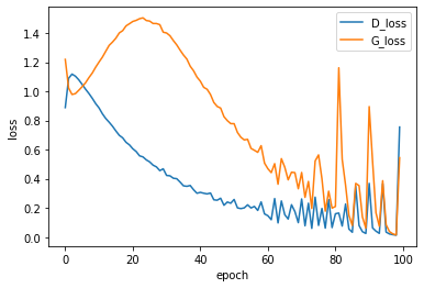
ロスは全然安定してないものの、generatorはまともなものを生成しているのでヨシ!とする
解釈器の実装
付録を見てもらえればわかるが、Generatorの特徴マップを抽出できるようにしている
def extract_features(self, z):
   z1 = self.fc1(z)
    z2 = self.fc2(z1)
    z2 = z2.view(-1, 128, 7, 7)
    z2 = self.deconv1(z2)
    x = self.deconv2(z2)
    return z, z1, z2, x
これらの特徴マップと出力を、新たな入力とし、少数アノテーションを教師として解釈器の学習を行う
解釈器は単純な構造のCNNを利用している
class Interpreter(nn.Module):
    def __init__(self):
        super(Interpreter, self).__init__()

        self.conv1 = nn.Sequential(
            nn.Conv2d(1, 64, kernel_size=4, stride=2, padding=1),
            nn.LeakyReLU(0.2)
        )

        self.conv2 = nn.Sequential(
            nn.Conv2d(64+64, 128, kernel_size=4, stride=2, padding=1),
            nn.BatchNorm2d(128),
            nn.LeakyReLU(0.2),
        )

        self.fc = nn.Sequential(
            nn.Linear(128 * 7 * 7*2 + 32, 1024),
            nn.BatchNorm1d(1024),
            nn.LeakyReLU(0.2),
            nn.Linear(1024, 10),
        )

        initialize_weights(self)

    def forward(self, x, z2, z1, z):
        h = self.conv1(x)
        h = self.conv2(torch.cat([h, z2], dim=1))
        h = h.view(-1, 128 * 7 * 7)
        h = self.fc(torch.cat([h, z1, z], dim=1))
        return h

def detach(*xs):
    return [x.detach() for x in xs]
生成器から100個のサンプルを取り出し、生成器に勾配が伝わらないようにdetachする
G = Generator().cuda()
G.load_state_dict(torch.load("./logs/MNIST_G_100.pth"))
G.eval()

def detach(*xs):
    return [x.detach() for x in xs]

with torch.no_grad():
    torch.manual_seed(42)
    sample_z = torch.randn((100, z_dim))
    sample_z = sample_z.cuda()

    z, z1, z2, x = G.extract_features(sample_z)
    z, z1, z2, x = detach(z, z1, z2, x)
    save_image(x.data.cpu(), os.path.join(log_dir, 'training_images.png'), nrow=10)
取り出した100個のサンプルにアノテーションを行う
5, 2, 9, 9, 9, …
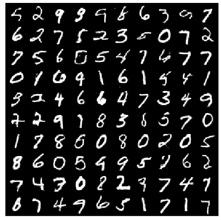
t = [
    5, 2, 9, 9, 9, 8, 6, 3, 5, 7,
    6, 2, 7, 5, 2, 3, 5, 0, 7, 2,
    7, 5, 6, 0, 5, 4, 7, 6, 7, 7,
    0, 1, 6, 4, 1, 6, 1, 5, 4, 1,
    3, 2, 4, 6, 6, 4, 7, 3, 4, 9,
    2, 2, 9, 1, 8, 3, 6, 5, 7, 0,
    1, 7, 8, 6, 0, 8, 9, 2, 0, 5,
    8, 6, 0, 5, 4, 9, 5, 7, 6, 2,
    7, 4, 3, 0, 8, 2, 3, 7, 4, 7,
    6, 7, 4, 9, 6, 5, 1, 7, 1, 7
    ]
10個の解釈器を上記の生成画像を使って訓練する
N = 10
Is = [Interpreter().cuda() for i in range(N)]
Is_opt = [optim.Adam(Is[i].parameters()) for i in range(N)]
criterion = nn.CrossEntropyLoss()
bs = 5
t = torch.tensor(t).cuda()
def train(optimizer, interpreter, z, z1, z2, x, t):
running_loss = 0.0
z, z1, z2, x, t = shuffle(z, z1, z2, x, t)
for i in range(int(len(t)/bs)):
z_, z1_, z2_, x_, t_ = z[bs*i:bs*(i+1)], z1[
bs*i:bs*(i+1)], z2[bs*i:bs*(i+1)], x[bs*i:bs*(i+1)], t[bs*i:bs*(i+1)]
optimizer.zero_grad()
y = interpreter(x_, z2_, z1_, z_)
loss = criterion(y, t_)
loss.backward()
optimizer.step()
running_loss += loss.item()
return running_loss/(len(t)/bs)
for opt, I in zip(Is_opt, Is):
for epoch in range(30):
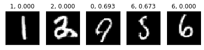
loss = train(opt, I, z, z1, z2, x, t)解釈器による予測を行い、多数決の結果と不確かさ(エントロピー)を画像の上に表示する
def interpreter_pred(Is, x, z2, z1, z):
    preds = []
    for I in Is:
        pred = I(x, z2, z1, z).argmax(1).detach().cpu().numpy()
        preds.append(pred)
    return np.array(preds)

for I in Is:
    I.eval()

sample_size = 5
with torch.no_grad():
    sample_z = torch.randn((sample_size, z_dim))
    sample_z = sample_z.cuda()

    z, z1, z2, x = G.extract_features(sample_z)
    z, z1, z2, x = detach(z, z1, z2, x)

    preds = interpreter_pred(Is, x, z2, z1, z)

plt.figure(figsize=(7, 2))
for i, x_ in enumerate(x.cpu().numpy()):
    plt.subplot(1, 5, i+1)
    plt.xticks([])
    plt.yticks([])
    hist, _ = np.histogram(preds[:, i], range(11), density=True)
    plt.title("{}, {:.3f}".format(hist.argmax(), entropy(hist)))
    plt.imshow(x_[0], cmap=plt.cm.gray)
plt.show()
不確かさが0だと解釈器の予測が割れていない状態を意味する
これで一旦「無限」データセット生成器が完成した
エントロピーが0.4以下(モデルが9つ以上同じ予測)のとき、データセットに加えることにする
def make_datasets(G, Is, M=1000, thresh=0.1, z_dim=32):
images = []
labels = []
sample_size = 64
for j in tqdm(range(M)):
with torch.no_grad():
sample_z = torch.randn((sample_size, z_dim))
sample_z = sample_z.cuda()
z, z1, z2, x = G.extract_features(sample_z)
z, z1, z2, x = detach(z, z1, z2, x)
preds = interpreter_pred(Is, x, z2, z1, z)
for i, x_ in enumerate(x.cpu().numpy()):
hist, _ = np.histogram(preds[:, i], range(11), density=True)
pred = hist.argmax()
ent = entropy(hist)
if ent < thresh:
images.append(x_)
labels.append(pred)
return np.array(images), np.array(labels)
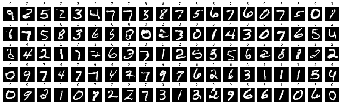
images, labels = make_datasets(G, Is)
plt.figure(figsize=(20, 6))
for i, (x_, y_) in enumerate(zip(images[:100], labels[:100])):
plt.subplot(5, 20, i+1)
plt.xticks([])
plt.yticks([])
plt.title(f"{y_}")
plt.imshow(x_[0], cmap=plt.cm.gray)
plt.show()画像の上の数字は解釈器で予測したラベル
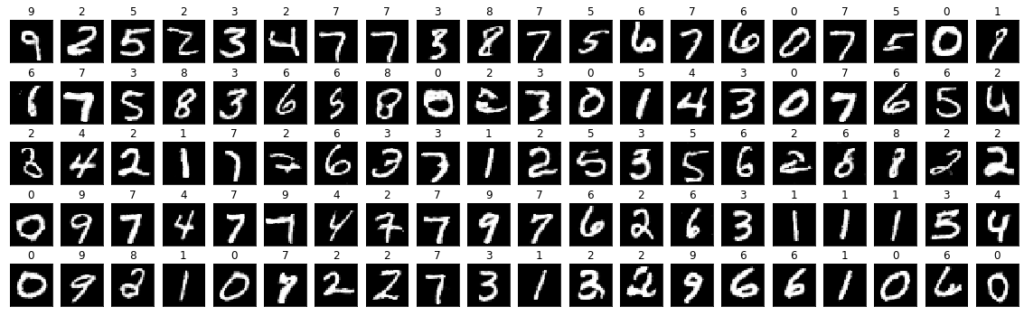
いくつか怪しいラベルが…
分類器の実装
単純なCNNった分類器を用意し、上記で作成したデータセットを使って訓練する
C = Classifier().cuda()
optimizer = optim.Adam(C.parameters())
C.train()

bs = 128
for epoch in range(30):
    running_loss = 0.0
    images, labels = shuffle(images, labels)
    for i in range(int(len(images)/bs)):
        x_, t_ = images[bs*i:bs*(i+1)], labels[bs*i:bs*(i+1)]

        optimizer.zero_grad()
        y = C(torch.from_numpy(x_).cuda())
        loss = criterion(y, torch.from_numpy(t_).cuda())
        loss.backward()
        optimizer.step()

        running_loss += loss.item()
    loss = running_loss/(len(t)/bs)
テストデータで分類器の評価を行う
dataset = datasets.MNIST("./data/mnist", transform=transform, train=False)
data_loader = torch.utils.data.DataLoader(dataset, batch_size=batch_size, shuffle=False)

C.eval()
pred = []
true = []
with torch.no_grad():
    for x_, t_ in data_loader:
        y = C(x_.cuda()).detach().cpu().numpy().argmax(1)
        pred.extend(y)
        true.extend(t_.numpy())

print(classification_report(pred, true))
confusion_matrix(pred, true)

# 出力
              precision    recall  f1-score   support

           0       0.85      0.92      0.88       900
           1       0.84      0.94      0.89      1013
           2       0.87      0.70      0.78      1282
           3       0.72      0.74      0.73       983
           4       0.69      0.91      0.78       745
           5       0.66      0.69      0.68       853
           6       0.95      0.74      0.83      1232
           7       0.82      0.82      0.82      1023
           8       0.81      0.86      0.83       919
           9       0.78      0.75      0.77      1050

    accuracy                           0.80     10000
   macro avg       0.80      0.81      0.80     10000
weighted avg       0.81      0.80      0.80     10000

array([[831,   0,   3,   5,   0,  16,   6,  10,  23,   6],
       [  1, 957,   0,   0,   8,   1,   0,  22,   4,  20],
       [ 22,  22, 899, 179,  35,   4,   8,  74,  25,  14],
       [  5,   1,   7, 727,   1, 142,   0,  22,  29,  49],
       [  0,   6,   1,   0, 676,   2,   1,   6,   5,  48],
       [ 21,  63,   3,  36,  21, 592,  30,  19,  35,  33],
       [ 79,  52,   8,  13,  29,  93, 911,   2,  37,   8],
       [  1,  21,  94,  10,  12,   2,   0, 838,  22,  23],
       [ 14,  11,  14,  33,   2,  35,   2,   1, 788,  19],
[ 6, 2, 3, 7, 198, 5, 0, 34, 6, 789]])全然精度でてないね。半教師あり学習なんだから98%近くでてもいいのに。
考察
結果は巷の半教師あり学習と比べて全然精度がでなかった
GANの特徴マップで得られる空間的成分を有効に活用したセグメンテーションのほうがDatasetGANを能力をいかすことができるのだろう
付録:GANの実装
import os
from os.path import join, exists
from glob import glob

from tqdm import tqdm

import matplotlib.pyplot as plt
import numpy as np

import torch
import torch.nn as nn
import torch.utils.data
import torch.optim as optim
from torch.nn import functional as F
from torchvision import datasets, transforms
from torchvision.utils import save_image

from sklearn.utils import shuffle
from sklearn.metrics import confusion_matrix, classification_report
from scipy.stats import entropy

batch_size = 128
lr = 0.0002
z_dim = 32
log_dir = './logs'

transform = transforms.Compose([
    transforms.ToTensor()
])
dataset = datasets.MNIST("./data/mnist", transform=transform, train=True)
data_loader = torch.utils.data.DataLoader(dataset, batch_size=batch_size, shuffle=True)

def initialize_weights(model):
    for m in model.modules():
        if isinstance(m, nn.Conv2d):
            m.weight.data.normal_(0, 0.02)
            m.bias.data.zero_()
        elif isinstance(m, nn.ConvTranspose2d):
            m.weight.data.normal_(0, 0.02)
            m.bias.data.zero_()
        elif isinstance(m, nn.Linear):
            m.weight.data.normal_(0, 0.02)
            m.bias.data.zero_()


def generate(epoch, G, log_dir='logs'):
    G.eval()

    if not os.path.exists(log_dir):
        os.makedirs(log_dir)

    torch.manual_seed(42)
    sample_z = torch.randn((64, z_dim))
    sample_z = sample_z.cuda()

    samples = G(sample_z).data.cpu()
    save_image(samples, os.path.join(log_dir, 'MNIST_epoch_%03d.png' % (epoch)))

class Generator(nn.Module):
    def __init__(self):
        super(Generator, self).__init__()

        self.fc1 = nn.Sequential(
            nn.Linear(z_dim, 1024),
            nn.BatchNorm1d(1024),
            nn.ReLU(),
            nn.Linear(1024, 128 * 7 * 7),
        )

        self.fc2 = nn.Sequential(
            nn.BatchNorm1d(128 * 7 * 7),
            nn.ReLU(),
        )

        self.deconv1 = nn.Sequential(
            nn.ConvTranspose2d(128, 64, kernel_size=4, stride=2, padding=1)
        )

        self.deconv2 = nn.Sequential(
            nn.BatchNorm2d(64),
            nn.ReLU(),
            nn.ConvTranspose2d(64, 1, kernel_size=4, stride=2, padding=1),
            nn.Sigmoid(),
        )

        initialize_weights(self)

    def extract_features(self, z):
        z1 = self.fc1(z)
        z2 = self.fc2(z1)
        z2 = z2.view(-1, 128, 7, 7)
        z2 = self.deconv1(z2)
        x = self.deconv2(z2)
        return z, z1, z2, x


    def forward(self, z):
        x = self.fc1(z)
        x = self.fc2(x)
        x = x.view(-1, 128, 7, 7)
        x = self.deconv1(x)
        x = self.deconv2(x)
        return x

class Discriminator(nn.Module):

    def __init__(self):
        super(Discriminator, self).__init__()

        self.conv = nn.Sequential(
            nn.Conv2d(1, 64, kernel_size=4, stride=2, padding=1),
            nn.LeakyReLU(0.2),
            nn.Conv2d(64, 128, kernel_size=4, stride=2, padding=1),
            nn.BatchNorm2d(128),
            nn.LeakyReLU(0.2),
        )

        self.fc = nn.Sequential(
            nn.Linear(128 * 7 * 7, 1024),
            nn.BatchNorm1d(1024),
            nn.LeakyReLU(0.2),
            nn.Linear(1024, 1),
            nn.Sigmoid(),
        )

        initialize_weights(self)

    def forward(self, input):
        x = self.conv(input)
        x = x.view(-1, 128 * 7 * 7)
        x = self.fc(x)
        return x

G = Generator().cuda()
D = Discriminator().cuda()

G_optimizer = optim.Adam(G.parameters(), lr=lr, betas=(0.5, 0.999))
D_optimizer = optim.Adam(D.parameters(), lr=lr, betas=(0.5, 0.999))

criterion = nn.BCELoss()

def train(D, G, criterion, D_optimizer, G_optimizer, data_loader):
    D.train()
    G.train()

    y_real = torch.ones(batch_size, 1).cuda()
    y_fake = torch.zeros(batch_size, 1).cuda()


    D_running_loss = 0
    G_running_loss = 0
    for batch_idx, (real_images, _) in enumerate(data_loader):
        if real_images.size()[0] != batch_size:
            break

        z = torch.normal(mean=torch.zeros(batch_size, z_dim), std=torch.ones(batch_size, z_dim))
        real_images, z = real_images.cuda(), z.cuda()

        # Discriminator
        D_optimizer.zero_grad()

        D_real = D(real_images)
        D_real_loss = criterion(D_real, y_real)

        fake_images = G(z)
        D_fake = D(fake_images.detach())
        D_fake_loss = criterion(D_fake, y_fake)

        D_loss = D_real_loss + D_fake_loss
        D_loss.backward()
        D_optimizer.step()
        D_running_loss += D_loss.item()

        # Generator
        z = torch.randn((batch_size, z_dim)).cuda()

        G_optimizer.zero_grad()

        fake_images = G(z)
        D_fake = D(fake_images)
        G_loss = criterion(D_fake, y_real)
        G_loss.backward()
        G_optimizer.step()
        G_running_loss += G_loss.item()

    D_running_loss /= len(data_loader)
    G_running_loss /= len(data_loader)

    return D_running_loss, G_running_loss

num_epochs = 100

history = {}
history['D_loss'] = []
history['G_loss'] = []
for epoch in range(num_epochs):
    D_loss, G_loss = train(D, G, criterion, D_optimizer, G_optimizer, data_loader)

    print('epoch %d, D_loss: %.4f G_loss: %.4f' % (epoch + 1, D_loss, G_loss))
    history['D_loss'].append(D_loss)
    history['G_loss'].append(G_loss)

    generate(epoch + 1, G, log_dir)
    if (epoch+1) % 50 == 0:
        torch.save(G.state_dict(), os.path.join(log_dir, 'MNIST_G_%03d.pth' % (epoch + 1)))
        torch.save(D.state_dict(), os.path.join(log_dir, 'MNIST_D_%03d.pth' % (epoch + 1)))
コメント